Weighted least-squares regression

This example begins with linear regression in the real domain and then builds up to show how linear problems can be thought of in the complex domain.

Useful references:

• https://stats.stackexchange.com/questions/66088/analysis-with-complex-data-anything-different

• https://www.chrishenson.net/article/complex_regression

import numpy as np
import matplotlib.pyplot as plt
from regressioninc.linear.models import add_intercept, OLS

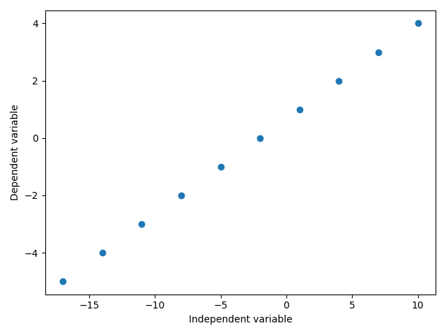
One of the most straightforward linear problems to understand is the equation of line. Let’s look at a line with gradient 3 and intercept -2.

params = np.array([3])
intercept = -2
X = np.arange(-5, 5).reshape(10, 1)
y = X * params + intercept

fig = plt.figure()
plt.scatter(y, X)
plt.xlabel("Independent variable")
plt.ylabel("Dependent variable")
plt.tight_layout()
fig.show()

When performing linear regressions, the aim is to:

• calculate the coefficients (coef, also called parameters)

• given the regressors (X, values of the independent variable)

• and values of the observations (y, values of the dependent variable)

This can be done with linear regression, and the most common method of linear regression is least squares, which aims to estimate the coefficients whilst minimising the squared misfit between the observations and estimated observations calculated using the estimated coefficients.

X = add_intercept(X)
model = OLS()
model.fit(X, y)
print(model.estimate.params)

[[ 3.]
 [-2.]]