Complex to real

Complex-valued linear problems can be reformulated as real-valued problems by splitting out the real and imaginary parts of the equations.

\[a + ib = C_1 (x + iy) .\]

Remember that we are solving for \(C_1 = (c_{1r} + c_{1i})\), which is also complex-valued, therefore,

\[a + ib = (c_{1r} + c_{1i}) (x + iy) .\]

This can be expanded out

\[\begin{split}a + ib &= (c_{1r} + ic_{1i}) (x + iy) \\ &= c_{1r} x - c_{1i} y + i c_{1r} y + i c_{1i} x \\ &= (c_{1r} x - c_{1i} y) + i (c_{1r} y + i c_{1i} x) ,\end{split}\]

which gives,

\[\begin{split}a &= c_{1r} x - c_{1i} y \\ b &= c_{1r} y + i c_{1i} x .\end{split}\]

For the complex-valued problem, the aim is to solve for \(C_1\). Making this real-valued means we are solving for \(c_{1r}\) and \(c_{1i}\).

Moving from complex-valued to real-valued results in the following

• Doubling the number of observations as the real and imaginary parts of the observations are split up

• Doubling the number of regressors as we are now solving for the real and imaginary component of each regressor explicitly

Usually, it is better to solve the problem with complex-values as outlined in this thread:

https://stats.stackexchange.com/questions/66088/analysis-with-complex-data-anything-different

import numpy as np
import matplotlib.pyplot as plt
from regressioninc.linear.models import add_intercept, OLS, MEstimator
from regressioninc.testing.complex import ComplexGrid, generate_linear_grid
from regressioninc.testing.complex import add_gaussian_noise
from regressioninc.testing.complex import add_outliers, plot_complex
from regressioninc.linear.models import complex_to_real, real_params_to_complex

np.random.seed(42)

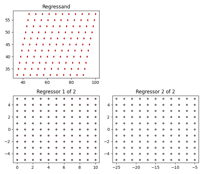
Let’s setup another linear regression problem with complex values

params = np.array([0.5 + 2j, -3 - 1j])
grid_r1 = ComplexGrid(r1=0, r2=10, nr=11, i1=-5, i2=5, ni=11)
grid_r2 = ComplexGrid(r1=-25, r2=-5, nr=11, i1=-5, i2=5, ni=11)
X, y = generate_linear_grid(params, [grid_r1, grid_r2], intercept=20 + 20j)

fig = plot_complex(X, y, {})
fig.set_size_inches(7, 6)
plt.tight_layout()
plt.show()

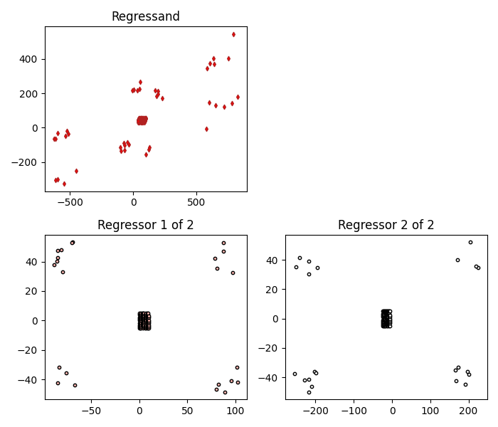
Add high leverage points to our regressors

seeds = [22, 36]
for ireg in range(X.shape[1]):
    np.random.seed(seeds[ireg])
    X[:, ireg] = add_outliers(
        X[:, ireg],
        outlier_percent=20,
        mult_min=7,
        mult_max=10,
        random_signs_real=True,
        random_signs_imag=True,
    )
np.random.seed(42)

intercept = 20 + 20j
y = np.matmul(X, params) + intercept

fig = plot_complex(X, y, {})
fig.set_size_inches(7, 6)
plt.tight_layout()
plt.show()

Solve

X = add_intercept(X)
model = OLS()
model.fit(X, y)
for idx, params in enumerate(model.estimate.params):
    print(f"parameter {idx}: {params:.6f}")

parameter 0: 0.500000+2.000000j
parameter 1: -3.000000-1.000000j
parameter 2: 20.000000+20.000000j

Add some outliers

y_noise = add_gaussian_noise(y, loc=(0, 0), scale=(21, 21))
model_ls = OLS()
model_ls.fit(X, y_noise)
for idx, params in enumerate(model_ls.estimate.params):
    print(f"parameter {idx}: {params:.6f}")

fig = plot_complex(X, y_noise, {"least squares": model_ls}, y_orig=y)
fig.set_size_inches(7, 9)
plt.tight_layout()
plt.show()

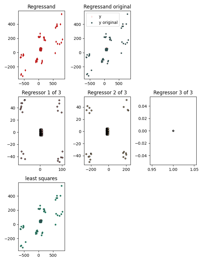
parameter 0: 0.504175+1.992051j
parameter 1: -3.002991-1.001990j
parameter 2: 19.634988+20.233521j

Add some outliers

y_noise = add_gaussian_noise(y, loc=(0, 0), scale=(21, 21))
model_mest = MEstimator()
model_mest.fit(X, y_noise)
for idx, params in enumerate(model_mest.estimate.params):
    print(f"paramsficient {idx}: {params:.6f}")

fig = plot_complex(
    X, y_noise, {"least squares": model_ls, "M estimate": model_mest}, y_orig=y
)
fig.set_size_inches(7, 9)
plt.tight_layout()
plt.show()

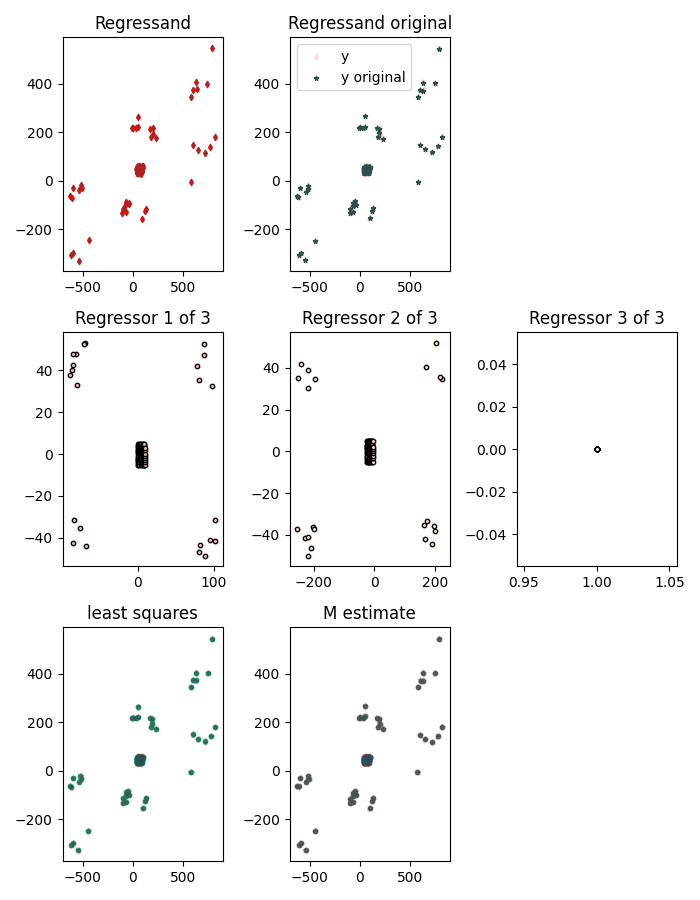
paramsficient 0: 0.509339+1.998580j
paramsficient 1: -2.999273-0.998400j
paramsficient 2: 20.362645+19.934598j

Try running as a real-valued problem

X_real, y_real = complex_to_real(X, y_noise)
model_ls = OLS()
model_ls.fit(X_real, y_real)
params = real_params_to_complex(model_ls.estimate.params)
for idx, params in enumerate(params):
    print(f"parameter {idx}: {params:.6f}")

parameter 0: 0.509492+1.998838j
parameter 1: -2.999218-0.998313j
parameter 2: 20.273556+19.907992j

Try running using real-valued M_estimates

model_mest = MEstimator()
model_mest.fit(X_real, y_real)
params = real_params_to_complex(model_mest.estimate.params)
for idx, params in enumerate(params):
    print(f"parameter {idx}: {params:.6f}")

parameter 0: 0.516664+1.999746j
parameter 1: -3.003042-1.001296j
parameter 2: 19.825662+19.956621j