Outliers

Outliers in data can occur for a variety of reasons. Depending on the ways in which they appear, they can be worth investigating in more detail. However, the presence of outliers can skew estimation of the parameters of interest.

More information about outliers:

• https://en.wikipedia.org/wiki/Outlier

import numpy as np
import matplotlib.pyplot as plt
from regressioninc.linear.models import add_intercept, OLS
from regressioninc.testing.complex import ComplexGrid, generate_linear_grid
from regressioninc.testing.complex import add_outliers, plot_complex

np.random.seed(42)

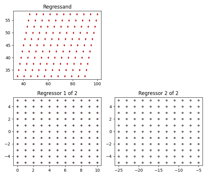
Let’s setup another linear regression problem with complex values.

params = np.array([0.5 + 2j, -3 - 1j])
grid_r1 = ComplexGrid(r1=0, r2=10, nr=11, i1=-5, i2=5, ni=11)
grid_r2 = ComplexGrid(r1=-25, r2=-5, nr=11, i1=-5, i2=5, ni=11)
X, y = generate_linear_grid(params, [grid_r1, grid_r2], intercept=20 + 20j)

fig = plot_complex(X, y, {})
fig.set_size_inches(7, 6)
plt.tight_layout()
plt.show()

Estimating the parameters using least squares gives the expected values.

X = add_intercept(X)
model = OLS()
model.fit(X, y)
for idx, params in enumerate(model.estimate.params):
    print(f"parameter {idx}: {params:.6f}")

fig = plot_complex(X, y, {"least squares": model})
fig.set_size_inches(7, 9)
plt.tight_layout()
plt.show()

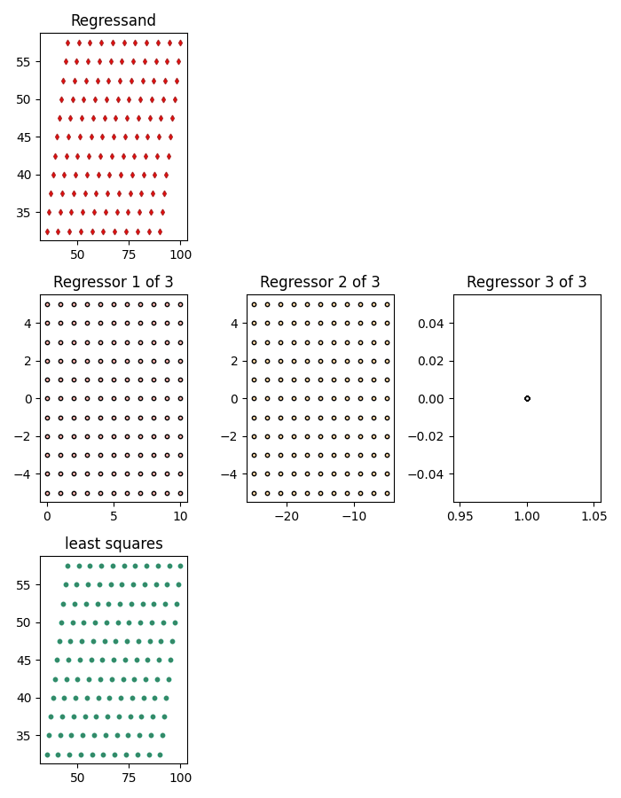
parameter 0: 0.500000+2.000000j
parameter 1: -3.000000-1.000000j
parameter 2: 20.000000+20.000000j

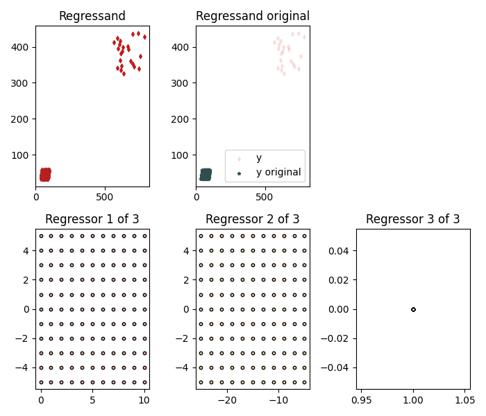
Add some outliers to the regrassands.

y_noise = add_outliers(y, outlier_percent=20, mult_min=5, mult_max=7)

fig = plot_complex(X, y_noise, {}, y_orig=y)
fig.set_size_inches(7, 6)
plt.tight_layout()
plt.show()

Now let’s try and estimate the parameters again but with the noisy regrassands. In this case, the parameter estimates are slightly off the actual value due to the presence of the noise.

model = OLS()
model.fit(X, y_noise)
for idx, params in enumerate(model.estimate.params):
    print(f"parameter {idx}: {params:.6f}")

fig = plot_complex(X, y_noise, {"least squares": model}, y_orig=y)
fig.set_size_inches(7, 9)
plt.tight_layout()
plt.show()

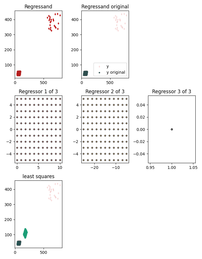
parameter 0: -4.696029+3.210866j
parameter 1: 1.053848-0.427605j
parameter 2: 219.256159+86.717843j