Multiple regressors

The previous example showed complex-valued regression with a single regressor. In practice, it is common to have multiple regressors. The following example will generate a complex-valued linear problem with multiple regressors and try and visualise it.

For those unfamiliar with these types of problems, please refer to the Wikipedia entry on linear regression.

• https://en.wikipedia.org/wiki/Linear_regression

from loguru import logger
import numpy as np
import matplotlib.pyplot as plt
from regressioninc.linear.models import add_intercept, OLS
from regressioninc.testing.complex import generate_random_regressors, plot_complex
from regressioninc.testing.complex import ComplexGrid

logger.remove()
np.random.seed(42)

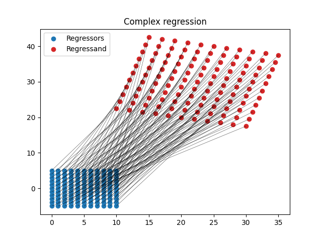
Let’s begin where the previous example ended.

grid = ComplexGrid(r1=0, r2=10, nr=11, i1=-5, i2=5, ni=11)
X = grid.flat_grid()
param1 = np.array([0.5 + 2j])
intercept = 20 + 20j
y = np.matmul(X, param1) + intercept

fig = plt.figure()
for iobs in range(y.size):
    plt.plot(
        [y[iobs].real, X[iobs, 0].real],
        [y[iobs].imag, X[iobs, 0].imag],
        color="k",
        lw=0.3,
    )
plt.scatter(X.real, X.imag, c="tab:blue", label="Regressors")
plt.grid()
plt.title("Regressors X")
plt.scatter(y.real, y.imag, c="tab:red", label="Regressand")
plt.grid()
plt.legend()
plt.title("Complex regression")
plt.show()

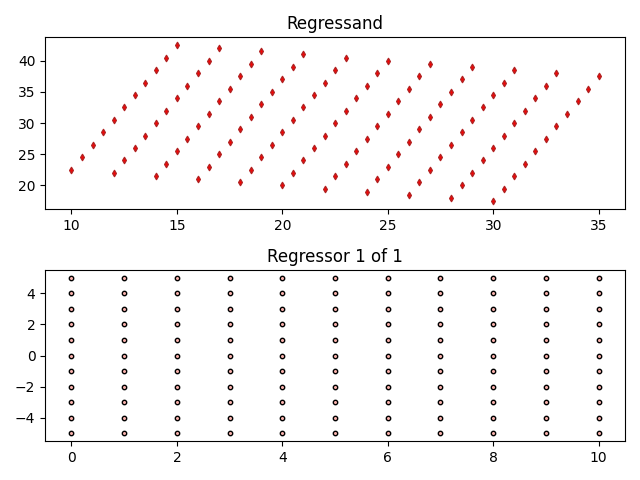
Now plot this in a different way that will make it easier to visualise more than a single regressor.

fig = plot_complex(X, y, {})
plt.show()

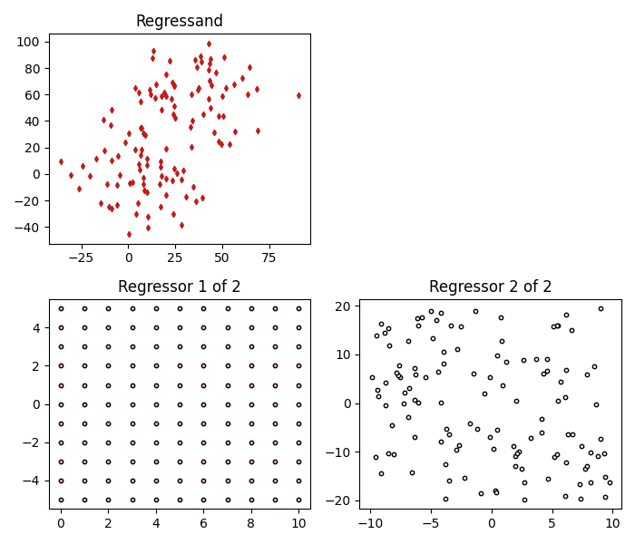
To add a second regressor, let’s define a second parameter (coefficent) and generate some random complex-valued data for the regressor.

param2 = np.array([2.7 - 1.8j])
X2 = generate_random_regressors(n_regressors=1, n_samples=y.size)

Now combine the new parameter and regressor data with the initial data and generate our new regrassand, which will also include an intercept.

params = np.concatenate((param1, param2))
X = np.concatenate((X, X2), axis=1)
intercept = 20 + 20j
y = np.matmul(X, params) + intercept

fig = plot_complex(X, y, {})
fig.set_size_inches(7, 6)
plt.tight_layout()
plt.show()

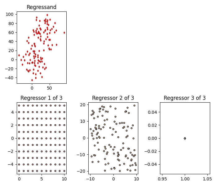
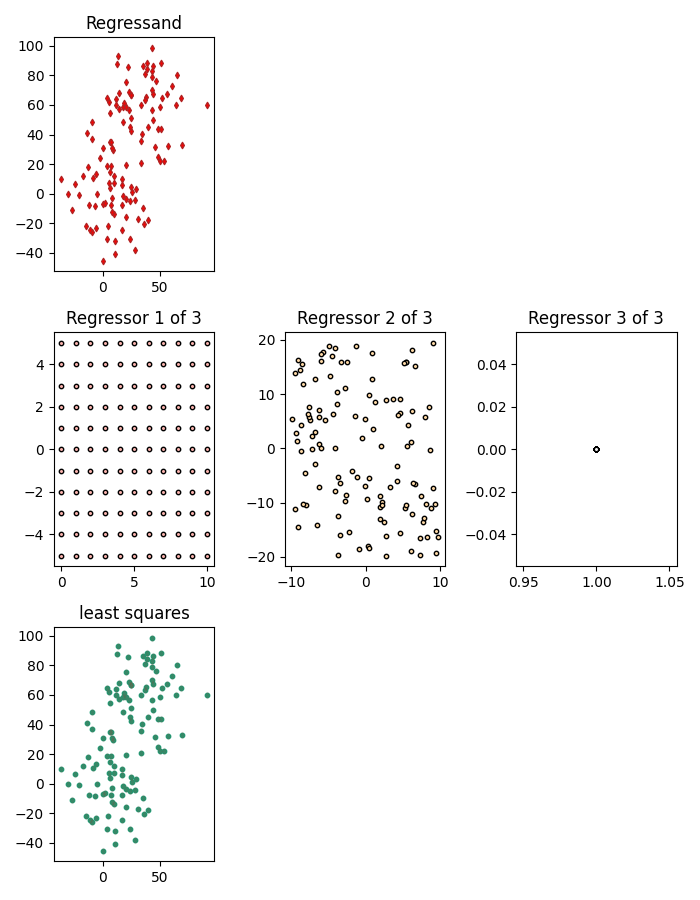
To solve for an intecerpt, an intercept column needs to be explicitly added to the regressors X before passing X through to the model. Adding an intercept simply adds a column of 1s to the regressors.

X = add_intercept(X)
fig = plot_complex(X, y, {})
fig.set_size_inches(7, 6)
plt.tight_layout()
plt.show()

Now the two parameters and the intercept can be estimated using the regrassand y and the regressors X and ordinary least squares.

model = OLS()
model.fit(X, y)
for idx, params in enumerate(model.estimate.params):
    print(f"parameter {idx}: {params:.6f}")

parameter 0: 0.500000+2.000000j
parameter 1: 2.700000-1.800000j
parameter 2: 20.000000+20.000000j

Finally, the predicted regressand calculated using the estimated parameters can be added to the visualisation.

fig = plot_complex(X, y, {"least squares": model})
fig.set_size_inches(7, 9)
plt.tight_layout()
plt.show()