Leverage points

Leverage points are large points in the regressors that can have a significant influence on coefficient estimates. High leverage points can be considered outliers with respect to independent variables or the regressors.

For more information on leverage points, see:

• https://en.wikipedia.org/wiki/Leverage_(statistics)

import numpy as np
import matplotlib.pyplot as plt
from regressioninc.linear import add_intercept, LeastSquares
from regressioninc.testing.complex import ComplexGrid, generate_linear_grid
from regressioninc.testing.complex import add_gaussian_noise, add_outliers, plot_complex

np.random.seed(42)

Let’s setup another linear regression problem with complex values.

coef = np.array([0.5 + 2j, -3 - 1j])
grid_r1 = ComplexGrid(r1=0, r2=10, nr=11, i1=-5, i2=5, ni=11)
grid_r2 = ComplexGrid(r1=-25, r2=-5, nr=11, i1=-5, i2=5, ni=11)
X, y = generate_linear_grid(coef, [grid_r1, grid_r2], intercept=20 + 20j)

fig = plot_complex(X, y, {})
fig.set_size_inches(7, 6)
plt.tight_layout()
plt.show()

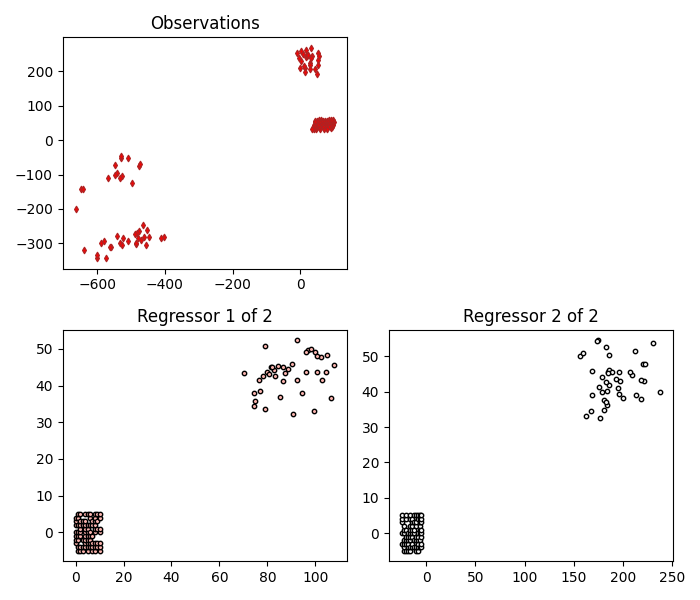
Add high leverage points to our regressors. Use different seeds for the two regressors to avoid getting the same outliers repeated twice.

seeds = [22, 36]
for ireg in range(X.shape[1]):
    np.random.seed(seeds[ireg])
    X[:, ireg] = add_outliers(
        X[:, ireg],
        outlier_percent=40,
        mult_min=7,
        mult_max=10,
        random_signs_real=False,
        random_signs_imag=False,
    )
np.random.seed(42)
intercept = 20 + 20j
y = np.matmul(X, coef) + intercept

fig = plot_complex(X, y, {})
fig.set_size_inches(7, 6)
plt.tight_layout()
plt.show()

Solve the regression problem. Note that there is no noise on the observations so whilst there are high leverage points in the regressors, everything is consistent.

X = add_intercept(X)
model = LeastSquares()
model.fit(X, y)
for idx, coef in enumerate(model.coef):
    print(f"Coefficient {idx}: {coef:.6f}")

Coefficient 0: 0.500000+2.000000j
Coefficient 1: -3.000000-1.000000j
Coefficient 2: 20.000000+20.000000j

As a next stage, add some outliers to the data and see what happens.

# y_noise = add_outliers(
#     y,
#     outlier_percent=20,
#     mult_min=7,
#     mult_max=10,
# )
y_noise = add_gaussian_noise(y, loc=(0, 0), scale=(5, 5))
model = LeastSquares()
model.fit(X, y_noise)
for idx, coef in enumerate(model.coef):
    print(f"Coefficient {idx}: {coef:.6f}")

fig = plot_complex(X, y_noise, {"least squares": model}, y_orig=y)
fig.set_size_inches(7, 9)
plt.tight_layout()
plt.show()

Coefficient 0: 0.500994+2.000610j
Coefficient 1: -2.999265-1.000917j
Coefficient 2: 19.781232+20.126984j